Support Vector Machine (SVM)
This SVM implementation classifies KOI objects as candidates or non-candidates using key transit, signal quality, and stellar features. The pipeline includes careful preprocessing, grid search tuning, and deployable artifacts.
Summary
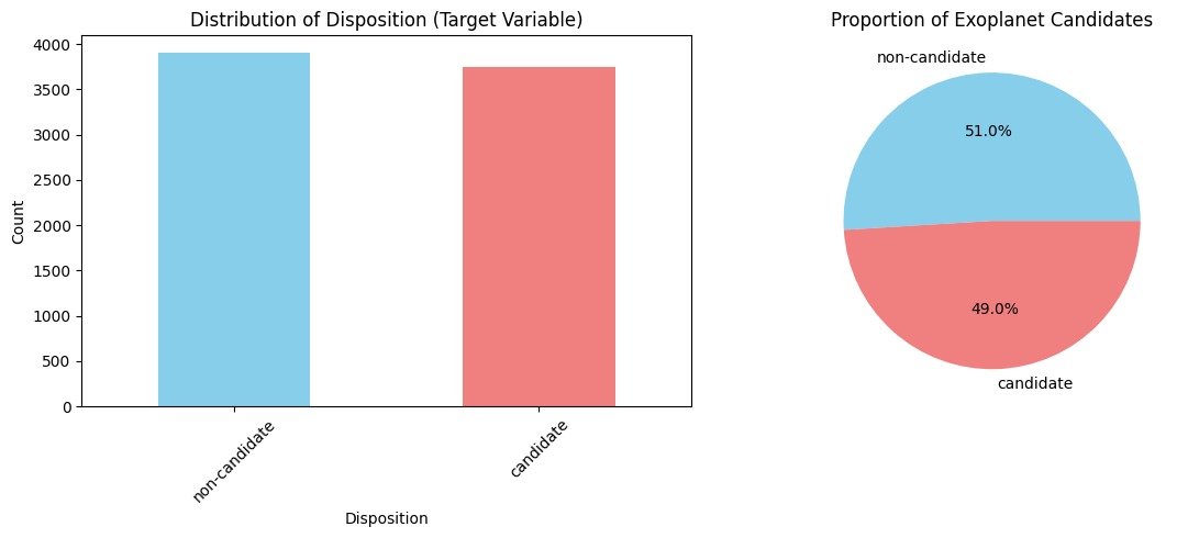
- Task: Binary classification of
koi_disposition - Kernels: RBF and Linear tested
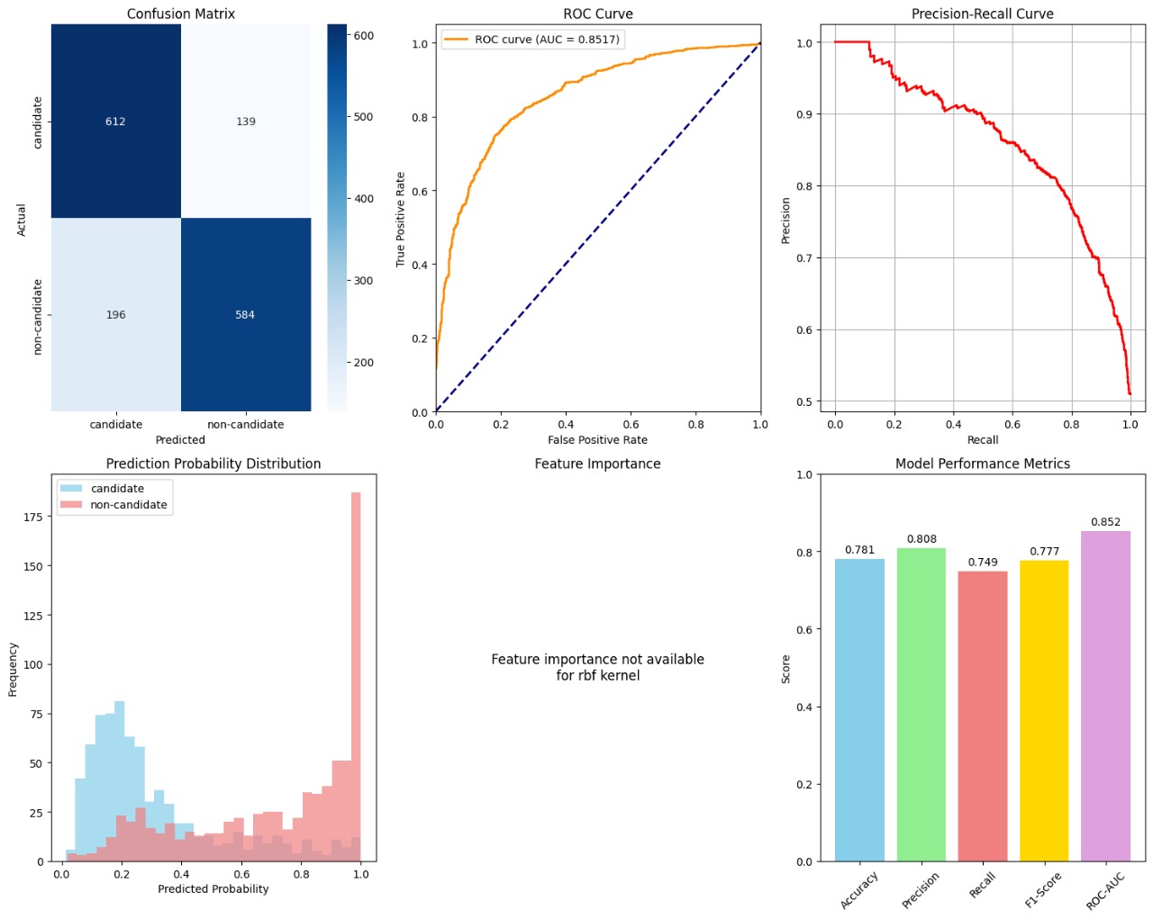
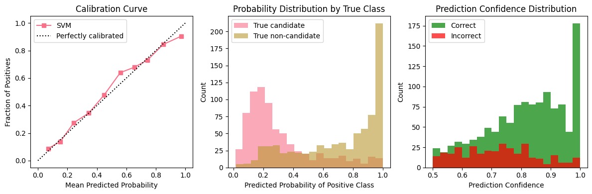
- Probability outputs enabled for confidence-based decisions
SVM theory (brief)
- Optimal separating hyperplane with maximum margin
- Support vectors define the decision boundary
- Kernel trick enables non-linear separation (RBF)
Optimization objective:
minimize: (1/2)||w||² + C∑ξᵢ subject to yᵢ(w·xᵢ + b) ≥ 1 - ξᵢ
Features and data
Representative feature set (see notebook for full list):
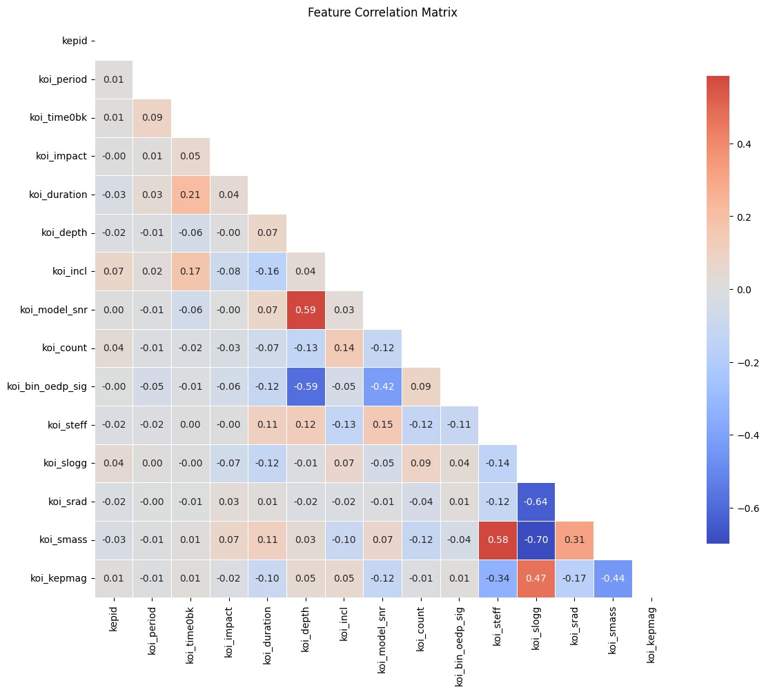
- Transit: koi_period, koi_duration, koi_depth, koi_impact
- Signal: koi_model_snr, koi_count, koi_bin_oedp_sig
- Stellar: koi_steff, koi_slogg, koi_srad, koi_smass, koi_kepmag
Preprocessing
- Missing values: median (numeric) / mode (categorical)
- Encoding: LabelEncoder for categoricals and target
- Scaling: StandardScaler (critical for SVM)
- Split: Stratified train/test (e.g., 80/20, random_state=42)
SVM draws a boundary between two classes. With the right settings, it handles non‑linear patterns well and gives clear decisions.
What it does
- Classifies
koi_dispositionas candidate vs non-candidate - Uses either a linear boundary or a flexible RBF boundary
When to use it
- You have KOI features in a table and want a strong baseline model
- You can scale features (SVM needs standardized inputs)
Data needed
- KOI features (period, duration, depth, SNR, etc.)
- Missing values filled (median), features scaled (StandardScaler)
How it works (simple)
- Scale all features to have similar ranges
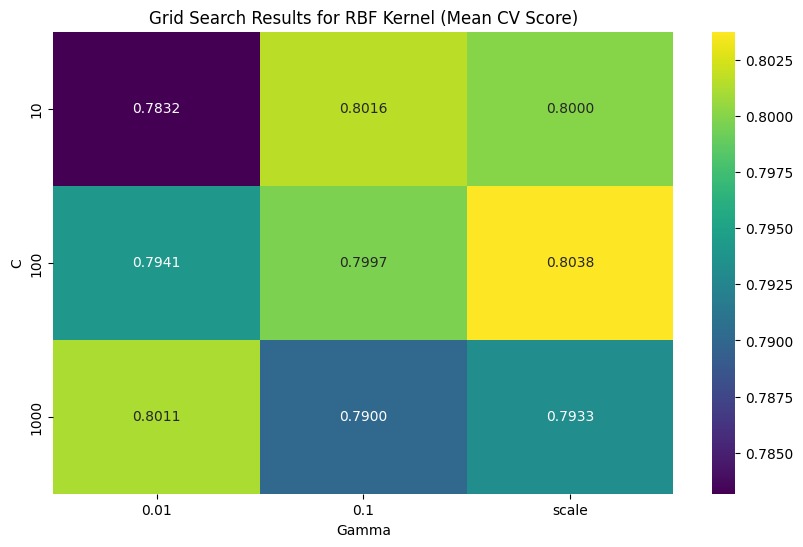
- Try different kernels (linear/RBF) and C/gamma values
- Pick the best settings via cross-validation and train the final model
What you’ll see (example visuals)
Outputs (files)
- Model + scaler + encoders saved with joblib
- Model metadata for tracking parameters and scores
Tips
- Always apply the same scaling at prediction time
- RBF often wins on non-linear data; linear is easier to interpret